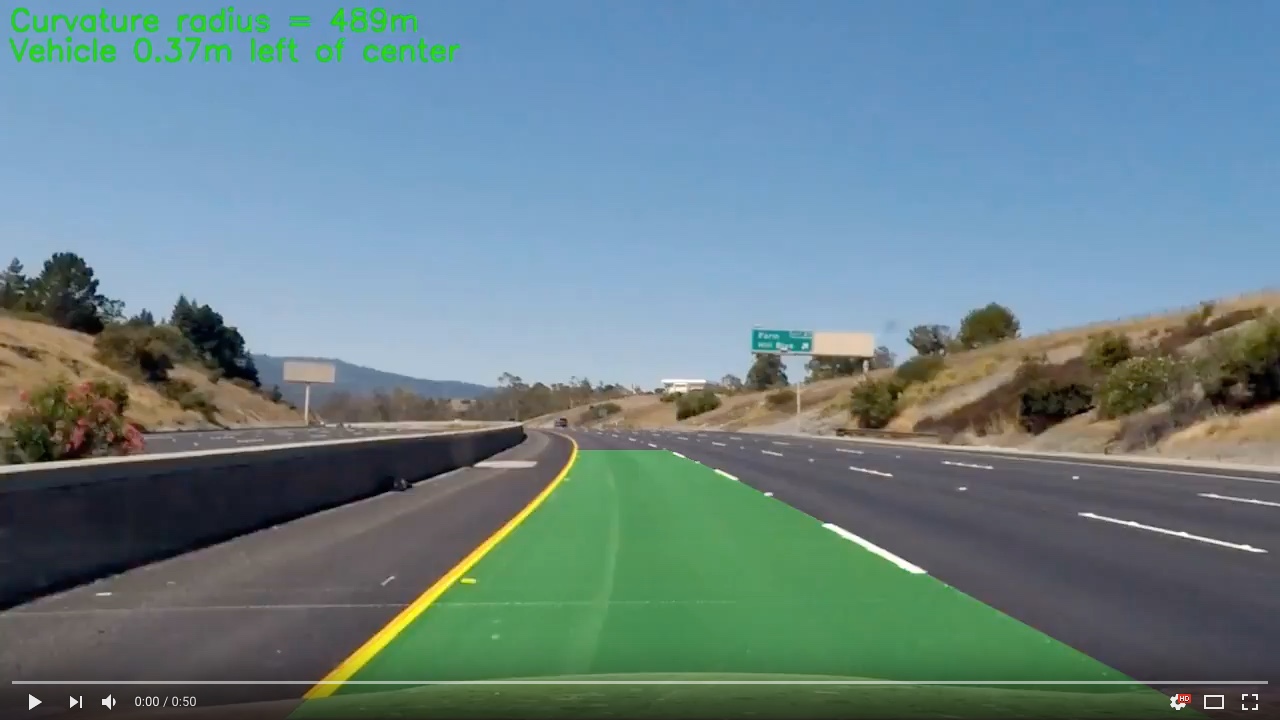
This is my submission for the Udacity Self-Driving Car Nanodegree Advanced Lane and Vehicle Detection Project. You can find my code in this Jupyter Notebook. Here I improve on my first Lane Detection Project by employing more advanced image thresholding and detection techniques as well as a linear Support Vector Machine (SVM) classifier to detect vehicles.
Summary
Prior to running the lane and vehicle detection pipelines, my code:
- Calibrates the camera
- Extracts feature vectors from vehicle and non-vehicle images
- Standardizes the feature vectors
- Splits the feature vectors into training and testing datasets
- Trains and tests a linear SVM using the datasets
Then a combined pipeline takes a video frame as its input, undistorts it, and passes it to the lane and vehicle detection pipelines.
Lane detection pipeline:
- Thresholds the image gradients and color spaces
- Combines the thresholded images
- Warps the combined image into a bird’s eye view perspective
- Detects the lane locations
- Calculates the road’s curvature radius and the vehicle’s relation to lane center
Vehicle detection pipeline:
- Scans a region of the video frame and extracts the feature vectors from the search window
- Standardizes the feature vectors
- Makes a prediction using the trained linear SVM
- Creates, thresholds, and separates a heatmap into individual regions
Finally, the combined pipeline draws the outputs of the lane and vehicle detection pipelines on the undistorted image.
Camera Calibration
A camera calibration matrix is computed which will be used to correct radial distortion caused by the camera lens.
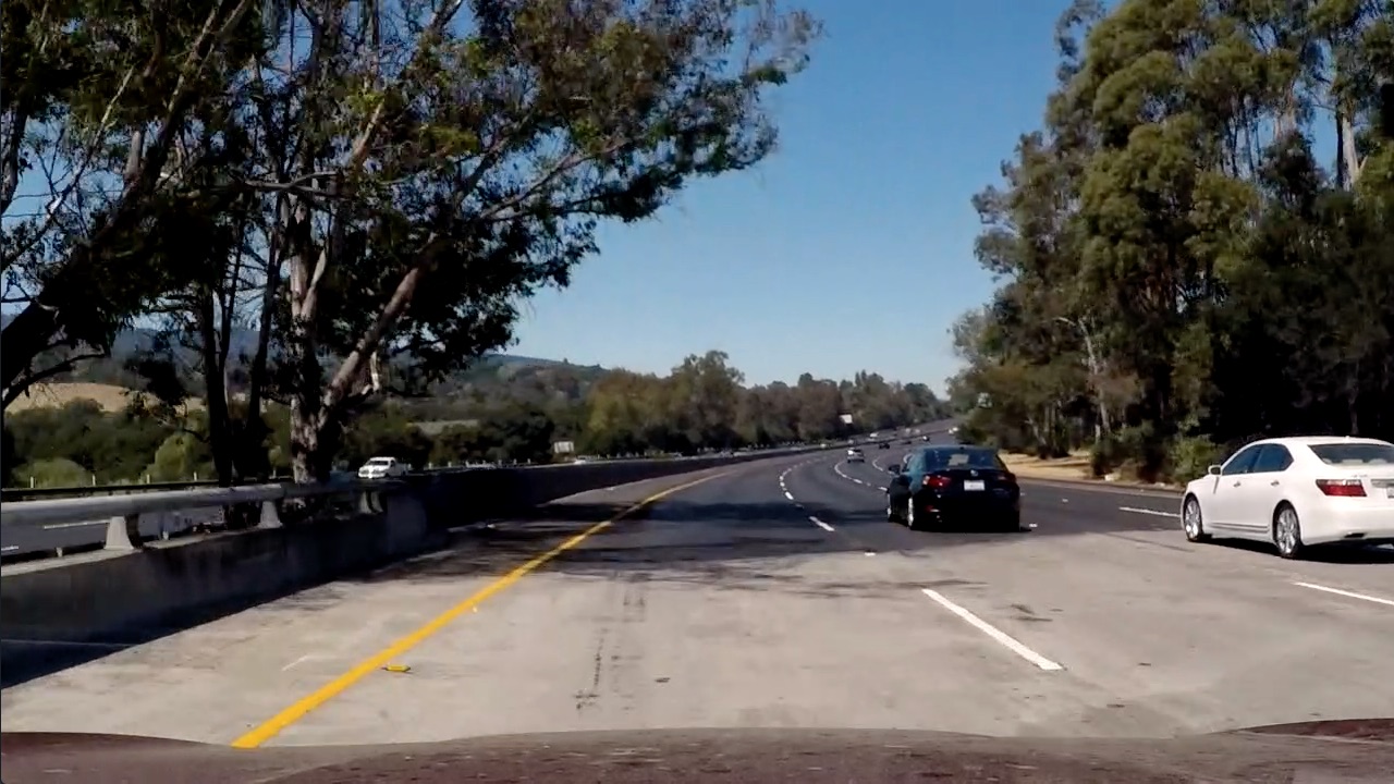
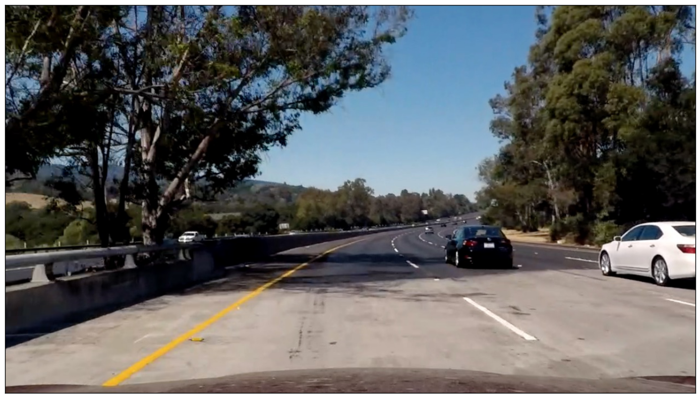
Images of a chessboard taken at various angles and distances are used to compute the camera calibration matrix. The chessboard inner corners are represented by a 9X6 matrix of coordinate object points. The calibration images are converted into grayscale and passed into cv2.findChessboardCorners which finds and outputs a matrix of coordinate image points. The object and image points are passed into cv2.calibrateCamera which outputs the camera calibration matrix. Finally, cv2.undistort is used to correct images taken with the same camera as the calibration images.
Chessboard calibration images:

A test image before distortion correction:
And after:
Dataset Compilation
The datasets that I used to train and test my classifier are made up of vehicle and non-vehicle images (64X64 pixels) from the GTI Vehicle Image Database and KITTI Vision Benchmark Suite.
First the images are converted from RGB to YCrCb before extracting their feature vectors. I experimented with different color spaces (RGB, HSV, HLS, YUV, LUV, and YCrCb) and found that the YCrCb color space yielded the best results in terms of positive vehicle detections.
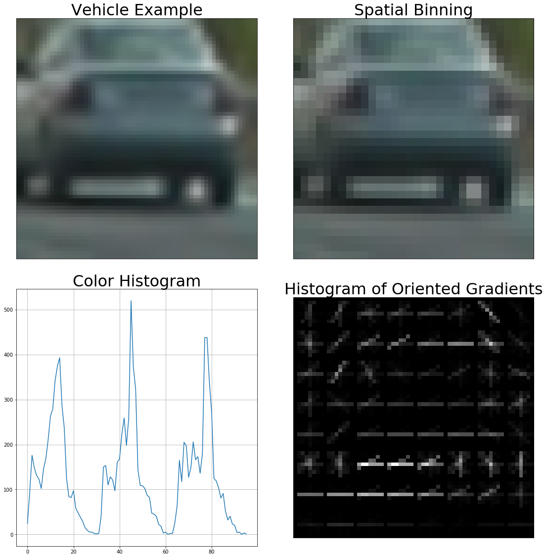
Next the spatial binning, color histogram, and Histogram of Oriented Gradients (HOG) feature vectors are extracted from the images. The spatial binning feature vector is a flattened, scaled down image; the image was scaled down to 32X32 pixels in my code. The idea behind spatial binning is that the scaled down image is less computationally expensive to process but still contains enough information to make a positive identification. The color histogram feature vector contains a color distribution which is unique to the area from which it was taken, therefore making it valuable information when making a prediction. The HOG feature vector also uses histograms, but in a clever way that allows for variability in the input image. The gradient directions in a cell (8X8 pixels in my code) are binned and their magnitudes summed. The gradient direction with the greatest summed magnitude is then normalized with its neighbors in a block (2X2 cells in my code). The resulting feature vector is less susceptible to variability because the gradients of several pixels are used.
The feature vectors are standardized by zero-mean centering and scaling to a standard deviation. They are then split into training and testing datasets (80/20 split in my code) which resulted in the following dataset sizes:
- Number of training examples = 14208
- Number of testing examples = 3552
Classifier Training
A linear SVM is trained and tested using the datasets defined in the previous section.
- Training Time = 32.683 s
- Training Accuracy = 1.000
- Testing Accuracy = 0.993
Lane Detection Pipeline
Gradient and Color Thresholding
In order to reliably detect the lanes in varying lighting and road surface conditions, several thresholds of the image gradients and color spaces are computed.
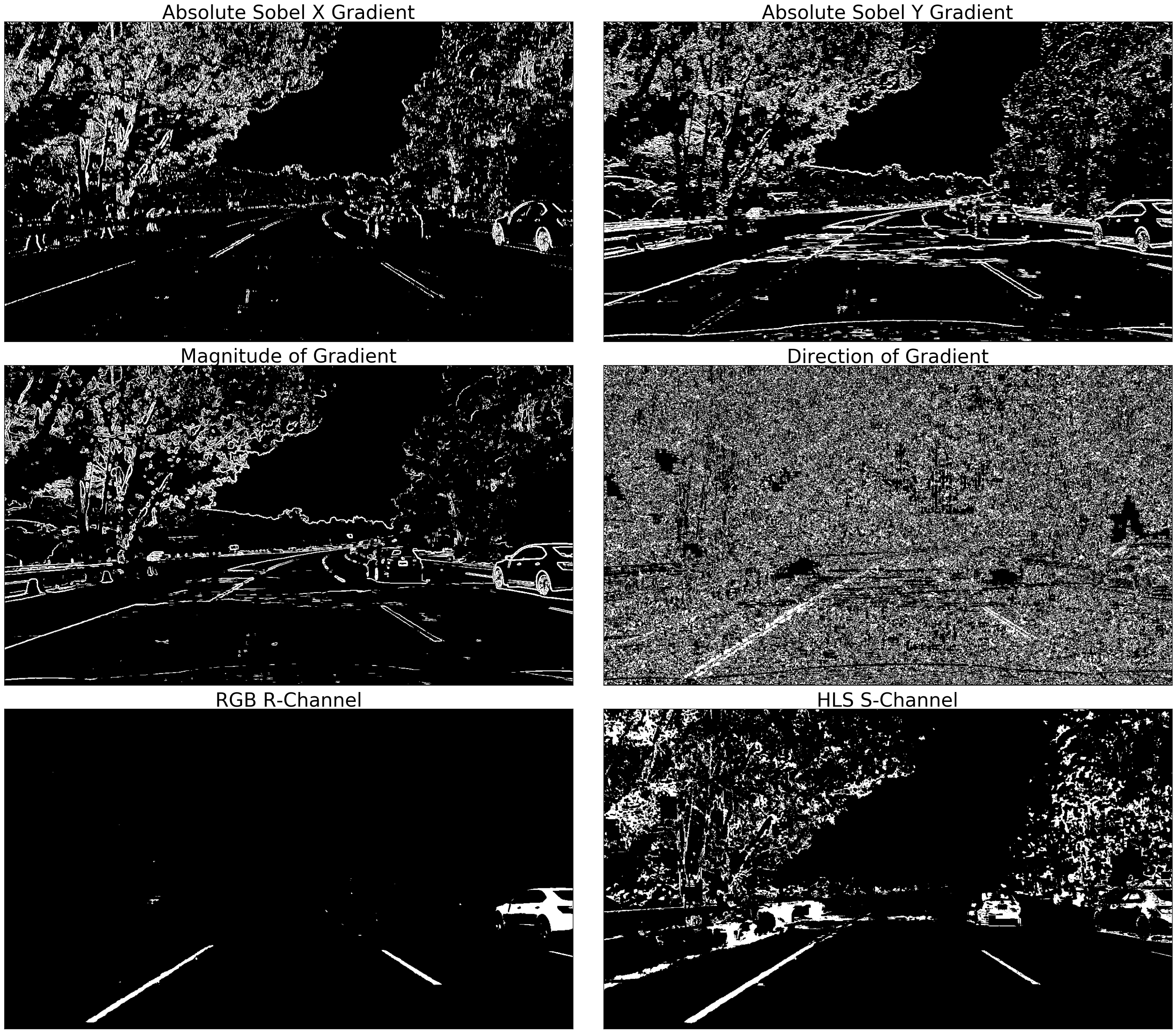
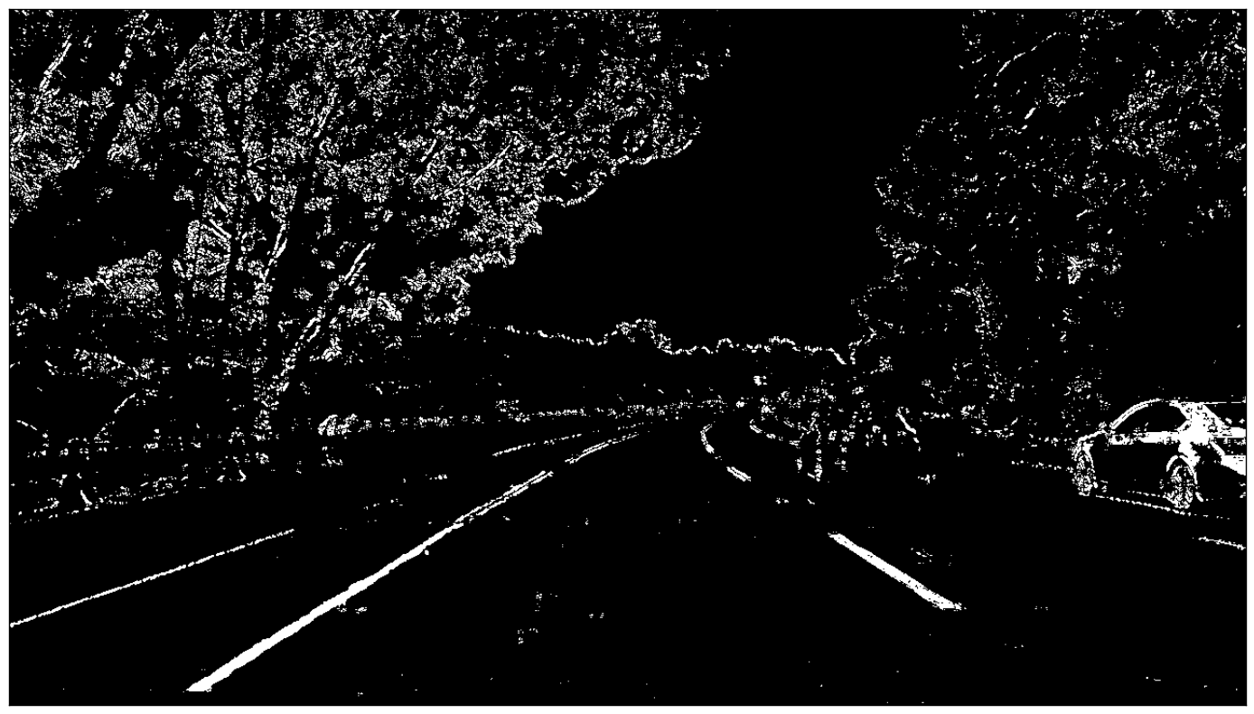
Once the thresholded binary images are computed they are combined using AND and OR operators:
binary_comb[((binary_gradx == 1) & (binary_grady == 1)) | ((binary_grad_mag == 1) & (binary_grad_dir == 1)) | ((binary_rch == 1) & (binary_sch == 1))] = 1
Warping
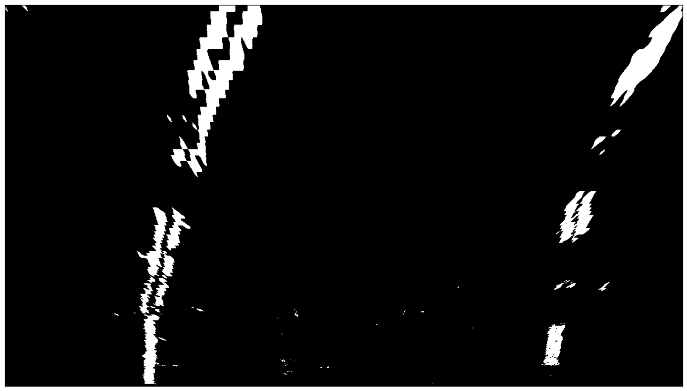
A bird’s eye view perspective shows the lane curvature more accurately than the driver’s perspective. The following source and destination points are used to compute a transformation matrix which is used to warp the image into the bird’s eye view perspective.
| Source Points | Destination Points |
|---|---|
| 685, 450 | 990, 0 |
| 1090, 720 | 990, 720 |
| 190, 720 | 290, 720 |
| 595, 450 | 290, 0 |

Warped image:
Lane Detection
A sliding window technique is used to identify the lanes in the first image that is passed through the pipeline. The starting points are identified by the peaks of a histogram evaluated at the bottom quarter of the image.
Histogram of bottom quarter of image:
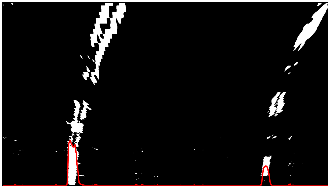
The following points are then identified by sliding the windows up from their starting points and locating the non-zero pixels that fall within the window bounds. The windows are centered on the average location of these non-zero pixels if their quantity is greater than a set threshold; if not, they are shifted by the previous amount. A polynomial is then fit to each set of left and right points.
Following the sliding window technique, the lanes are identified by locating all non-zero points that fall within the previously computed polynomials +/- a margin. A polynomial is then fit to each set of left and right points.
To smooth the results I computed a weighted average of the current and previous polynomial coefficients. For the weights I used the fraction of detected non-zero pixels for the current and previous image.
The current and previous polynomial coefficients are compared and saved if they fall within a margin of each other. Otherwise, the lanes are identified from scratch using the sliding window technique.
Road Curvature Radius and Vehicle Relation to Lane Center
I used the polynomial coefficients to compute the road’s curvature radius at the bottom of the image. I also compute the vehicle’s relation to lane center by subtracting the lane center from half of the image width (vehicle center).
Vehicle Detection Pipeline
Vehicle Detection
A sliding search window is used to find vehicles in the video frames. The search area is bounded to the lower half of the video frame because we don’t have to worry about flying cars… yet. Because the linear SVM classifier was trained on feature vectors extracted from 64X64 pixel images, the feature vector that is fed into the classifier must be extracted from a search window that matches those dimensions, therefore scaling is done before cropping. I found that the vehicles in the video are roughly 1.25 to 1.50 times the size of the training images when a reasonable distance away and up close.
To increase the frames/second processing time of my pipeline, the HOG feature vector is extracted only once per scale from the region of interest in the video frame (lower half). The HOG feature vector is split into a sub feature vector by cell coordinates as defined by the search window. A corresponding search window is cropped from the region of interest and the spatial binning and color histogram features are extracted from it. The three feature vectors are then combined and fed into the trained linear SVM classifier which outputs a prediction along with its measure of confidence. The first level of false positive filtering is done by discarding predictions with a measure of confidence of less than 0.5 (a positive number indicates a possible vehicle detection) and saving the search window coordinate points of all other predictions.
Heat Mapping
A heatmap is created to further discard false positives and combine multiple detections. The bounding boxes are filled in on a blank canvas of the same shape as the video frames; this is done over a series of 4 frames and continuously updated to yield detections that are more robust when compared to those made using a single frame. The resulting heatmap is then thresholded such that any pixels having an intensity of less than 4 are set to 0. This means that any detections that were made less than 4 times are discarded.
Results
The combined pipeline uses the outputs of the lane and vehicle detection pipelines to draw the highlighted lane, road’s curvature radius, vehicle’s relation to lane center, and vehicle bounding boxes on the undistorted image.
Conclusion
I spent a lot of time tweaking the image gradient and color space thresholds as well as different combinations of thresholded binary images. With more time I would be able to better optimize the parameters so that the pipeline would be able to generalize on the project and challenge videos.
I also tried different lane validation criteria, such as comparing lane curvature and detection confidence, but settled on a simple approach of comparing the polynomial coefficients to determine whether a lane was correctly detected.
I plan on revisiting this project to improve the robustness of my pipeline so that it could successfully detect the lanes in the challenge videos. I would also like to implement an idea that I have to track the vehicles once they have been detected.
References
Udacity Self-Driving Car ND - Term 1 Starter Kit
Udacity Self-Driving Car ND - Advanced Lane Detection Project
